Next: Software for GMSE analysis Up: Generalized Multiscale Entropy (GMSE) Analysis: Quantifying the Structure Previous: MSE and MSE analysis of RR interval time
Long-term trends change the overall but not the local SD/variance of a time series. As a consequence trends affect mostly MSEμ not MSEσ when the r value is calculated as a percentage of the time series’ SD. MSEμ and MSEσ values are much less effected by trends in implementations that use a fixed r value.
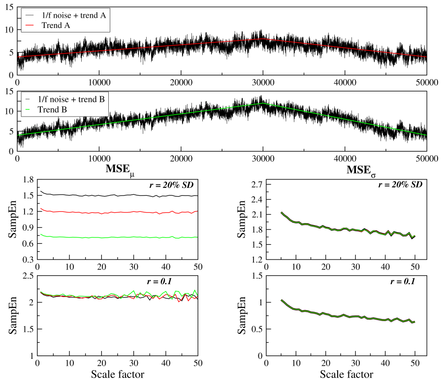
Figure 4 illustrates the effects that linear trends superimposed on normalized 1/f noise fluctuations have on MSEμ and MSEσ values. We considered trends obtained by the concatenation of two linear segments. In one case (red line) the values of the function increase linearly between 4 and 8 for the first 30,000 and then decrease linearly from 8 to to 4 over the following 20,000 data points. In the other case (green line), the rates of increase/decrease were doubled. The superimposition of each of these trends on a 1/f noise time series resulted in signals A and B shown on the first and second panels, respectively.
|
The SD of the original 1/f noise time series is one. The SDs of time series A and B are 1.3 (30% larger than the SD of the original series) and 2.3 (130% larger than the SD of the original series), respectively.
In MSEμ analyses using the 20% of SD criterion, the absolute values of r are 0.2, 0.26 and 0.46 for the original, time series A and B, respectively. The increase in the absolute value of r due to the trends results in a higher number of matches and consequently in lower entropy values. Specifically, for scale 1, in the case of 1/f noise, the number of matches with m = 2 and m = 3 were 28,348,070 and 5,827,479, respectively. For time series A (B), the number of matches with m = 2 and m = 3 were 38,606,695 (60,511,987) and 10,973,294 (27,887,816), respectively. The effects of trends on MSEμ can be obviated by using a fixed r value. However, when using r = 20% of SD, a barely noticeable trend can significantly change the values of entropy.
In MSEσ analysis, the r value is a percentage of the SD of the SD coarse-grained time series obtained with a window of 5 data points. Since the slow trend has only a small effect on the SD coarse-grained time series, the changes in the entropy values are negligible.
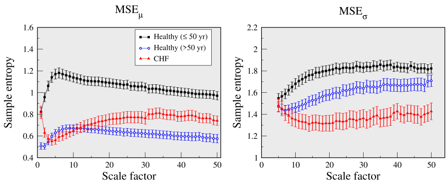
Figure 5 shows the results of MSEμ and MSEσ analyses of the RR interval time series from the groups of healthy young and older subjects and patients with CHF, using r = 20% SD. The first 50,000 data points of each recording (≈ 14-hours) were selected for analysis independent of the starting time (not available in most of these cases). As such, the time series may include both awake and sleep periods.
|
Healthy individuals are more likely to have more pronounced circadian variations than patients with CHF. Thus, the RR interval time series from the former group are more likely to exhibit trends of higher amplitude than the latter. These trends can justify the apparent contradictory MSEμ results that indicate higher dynamical complexity for the CHF than the healthy older group. Such a conjecture is supported by the MSEμ results obtained using a fixed r value as well as the those of MSEσ analyses using both fixed and variable r values. These findings highlight the need to analyze the data using different approaches in order to gain a deeper understanding of the properties of the dynamics and minimize the impact of known and unsuspected confounders.
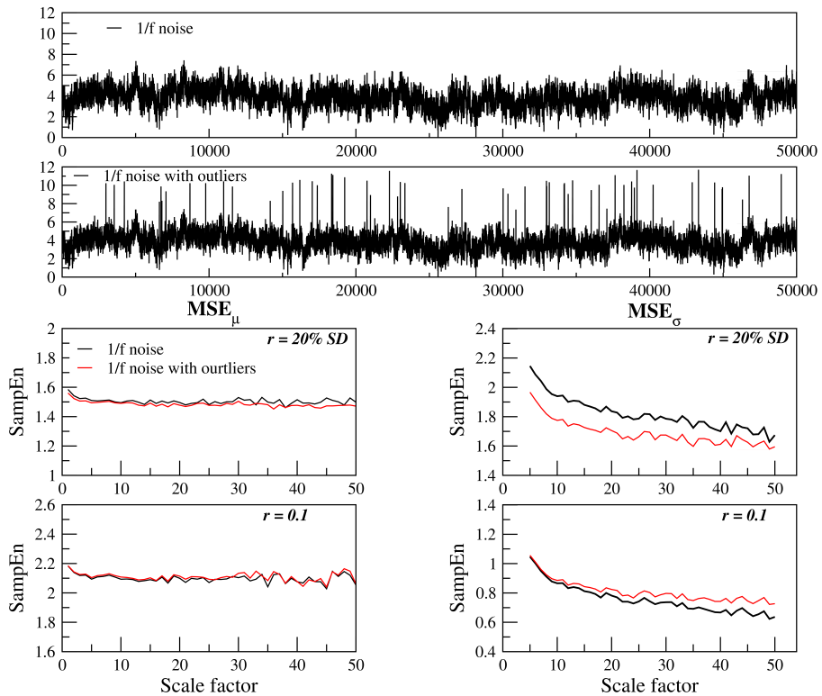
The presence of outliers can also significantly affect MSEσ, MSEσ2 and MSEMAD analyses. For this reason it is important to filter the time series prior to performing these analyses. The results presented here of the RR interval time series analyses were obtained using the filter described below. Alternatively, the use of a metric such as median absolute deviation for coarse-graining (not implemented here) could be considered.